If you’re starting your Data Science or Machine learning journey, Linear Regression might be the very first Machine Learning Algorithm or Statistical model you might be learning. It’s perhaps one of the simplest and most well-known algorithms in Machine Learning and Statistics. Here we’ll be exploring the simple linear regression and its key ideas intuitively along with the pseudo-code and python implementation.

Before getting to Linear Regression or any kind of regression per se, it’s crucial to understand the concept of Regression Modeling. In the field of statistics, Regression Modeling is a methodology for formulating the mathematical relationship between a dependent variable and a set of independent variables. For instance, you want to estimate the weight of certain individuals, which is affected by their diet, height, and exercise habits. Here, weight is the dependent variable (outcome), and the rest three are independent variables (predictors).

Is Linear Regression a Statistical Algorithm?

The goal of machine learning, and more specifically predictive modeling is to minimize the error by making the best predictions while skimming on the explainability. In applied machine learning, we utilize algorithms from a variety of fields (majorly statistics) for these purposes. Therefore, linear regression originated in the field of statistics in order to understand the relationship between input and output numerical variables, but engineering has borrowed it for machine learning. Hence, in addition to being a statistical algorithm, it’s also a machine learning algorithm. Now, let’s understand what it’s all about.

Defining Linear Regression

Linear regression is a powerful supervised machine learning algorithm that assumes a linear relationship between the dependent and independent variables. It’s simply the processor of finding the best fitting line that most accurately explains the variability between dependent and independent features. Let’s assume linear regression to be a vending machine that takes an input variable (predictor) x and returns an output variable(outcome) y. If there’s only one input variable or feature, we call it Simple Linear Regression and if there are multiple input variables, we call it Multiple Linear Regression. There are many equations to represent a straight line but we’ll stick with the following equation:

$$ \begin{equation} {y}_i = {\beta}_0 + {\beta}_1x_i \end{equation} $$

Here βo is the y-intercept and β1 is the slope. Let’s try to understand it with the help of a diagram.

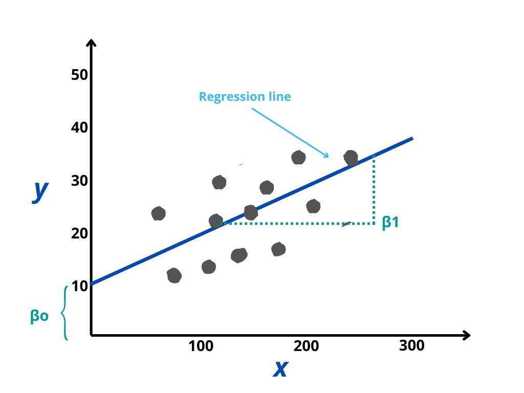
In the above diagram:

• The x-axis plots our independent variable x and the y-axis lots our dependent variable y
• Data points (actual values) are represented by the gray dots here
• βo is the intercept which is 10 and β1 is the slope of the x variable.
• Based on our model, the blue line is the best fit line, which corresponds to the predicted values
• An error or residual is a measure of how far a data point is from the regression line i.e it’s simply the deviation from our model

As we know from the theory that the equation for linear regression contains two coefficients i.e βo which is the intercept and β1 - the slope. In order to get the best-fit line, we must calculate these coefficients and the algorithm for this is mentioned below.

Pseudocode for Simple Linear Regression

1. Start

2. Read Number of Data (n)

3. For i=1 to n:
     Read Xi and Yi
   Next i

4. Initialize:
     sumX = 0
     sumX2 = 0
     sumY = 0
     sumXY = 0

5. Calculate Required Sum
   For i=1 to n:
     sumX = sumX + Xi
     sumX2 = sumX2 + Xi * Xi
     sumY = sumY + Yi
     sumXY = sumXY + Xi * Yi
   Next i

6. Calculate Required Constant a and b of y = a + bx:
   b = (n * sumXY - sumX * sumY)/(n*sumX2 - sumX * sumX)
   a = (sumY - b*sumX)/n

7. Stop

Linear Regression Algorithm in Practice Using Python

Having covered the theory, let’s learn how we can do it in practice using python. Python’s advantage is that we don’t have to implement popular Machine Learning Algorithms from scratch. There are python libraries for everything from Machine Learning to data visualization, with a very active community of developers. We’ll be using the Scikit Learn library to develop our Linear regression model.

A great feature of the SciKit Learn Library is that it includes toy datasets, making it easy for new users to practice before tackling more complex problems. We’ll be using the diabetic dataset for our demonstration of the linear regression model.

Step-1: Importing the libraries

We’ll start by importing the relevant libraries, some of the very important ones are:

• NumPy (to perform certain mathematical operations)
• pandas (to storethe data in a pandas DataFrames)
• matplotlib.pyplot (we will use matplotlib to plot the data along with seaborn)

import matplotlib.pyplot as plt
import numpy as np
import pandas as pd
import seaborn as sns
from sklearn import datasets, linear_model
from sklearn.metrics import mean_squared_error, r2_score

Step-2: Loading the Dataset

Our next step will be to import the data into a DataFrame. A DataFrame is an object in python that will help us keep our data organized in a tabular format. Let’s now load the data from sklearn’s diabetes dataset and create our dataframes.

# Load the diabetes dataset
diabetes_X, diabetes_y = datasets.load_diabetes(return_X_y=True)

# Create dataframe and add column names
features = pd.DataFrame(diabetes_X, columns=["age","sex","bmi","bp", "tc", "ldl", "hdl","tch", "ltg", "glu"])
target = pd.DataFrame(diabetes_y, columns=["disease_progression"])
df = pd.merge(features,target, left_index=True, right_index=True)

Step-3: Visualization

Let us now plot a heatmap for all the variables in order to find some correlation in our dataset to get the intuition.

correlation_matrix = df.corr()
f, ax = plt.subplots(figsize=(12, 9))
sns.heatmap(correlation_matrix, vmax=.8, square=True);

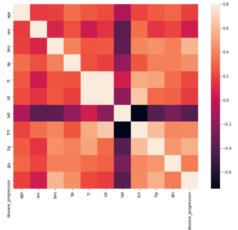
As we can see from the heatmap, age and disease_progression have a higher correlation as compared to other variables. You can go ahead and play with the visualizations and can find out interesting insights from the data.

Step 4: Performing Simple Linear Regression

At first, we need to split the dataset into training and testing datasets. We’ll be training our model using the training dataset and then validating our model using the testing dataset.

# Split into validation and training data
diabetes_X_train, diabetes_X_test, diabetes_y_train, diabetes_y_test = train_test_split(features, target, test_size=0.1, random_state=1)

Now that we have our training and testing datasets, we’ll create a LinearRegression object using sklearn’s linear_model and train our model with the training dataset.

# Create linear regression object
regr = linear_model.LinearRegression()

# Train the model using the training sets
regr.fit(diabetes_X_train, diabetes_y_train)

After our model has been trained we’ll evaluate our model by validating it against the test data sets as follows

# Make predictions using the testing set
diabetes_y_pred = regr.predict(diabetes_X_test)

# The coefficients
print("Coefficients: \n", regr.coef_)
# The mean squared error
print("Mean squared error: %.2f" % mean_squared_error(diabetes_y_test, diabetes_y_pred))
# The coefficient of determination: 1 is perfect prediction
print("Coefficient of determination: %.2f" % r2_score(diabetes_y_test, diabetes_y_pred))

In the above example, the Mean Squared Error measures how close a regression line is to a set of data points i.e. how close the observed data points are to the predicted values. Mean square error is calculated by taking the average, specifically the mean, of errors squared from data as it relates to a function. Mathematically it can be represented as,

$$ \sum_{i=1}^{D}(y_i-\hat{y}_i)^2 $$

Mean Squared Error and r2 Score are closely related but aren’t identical. It can be defined as “(total variance explained by the model) / total variance”. R-squared is a better measure than MSE. Because the value of Mean Squared Error depends on the units of the variables (i.e. it is not a normalized measure), it can change with the change in the unit of the variables.

Conclusion

Having covered the most fundamental concepts of Linear Regression and in fact Machine Learning, it’s time for you to pick up a dataset and put your learning into practice. Kaggle is a great place for getting started! Hope you had fun, see you next time!